“How are you doing at your new company?” - Me
“Really well, I finally learned how to use vlookups and PivotTables!” – Anonymous Friend
Valuable Skills
It is widely accepted that data analysis is an essential function for any healthy business. However, it is not easy to understand what data analysis is and how it’s useful. In the past, when I heard the term “data anaylsis,” I pictured an old man with puffy white hair poring over complicated mathematical formulas and giant sheets of unreadable numbers. Since then, I have learned that basic data analysis is not very complicated, and anyone with a simple computer and Excel can crank out some compelling stuff.
This post is written for all those people who have realized the value of vlookups, but hate its quirkiness. Microsoft has a free add-in for Excel 2010 called PowerPivot. This add-in puts enterprise grade database features within reach of Excel users. Let’s see how PowerPivot kills the need for vlookups, and does it with flying colors.
The Coffee Company Conundrum
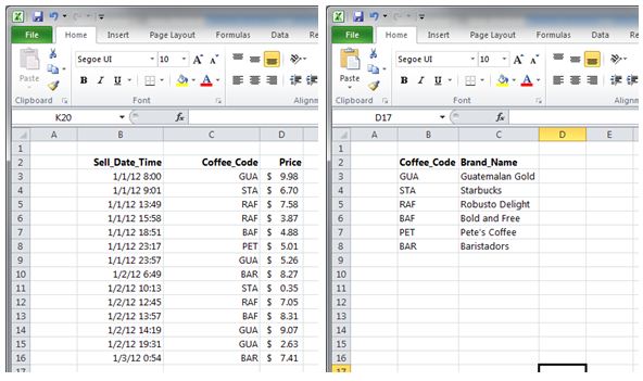
Let’s imagine we operate a small coffee shop. Every time a customer makes a purchase, it is recorded in some kind of computer system. As a manager, we want to see what types of coffee have been selling so we can better predict when and what we need to order. We are also interested in seeing the profitability of each of our brands.
Suppose our IT guy hands us two Excel sheets that look like this:
Step 1 – Make Tables
First we want to “tell” Excel that we are working with tables of data. We do the following steps for both the tables:
1. Click the Insert tab
2. Click somewhere in the table
3. Click Table
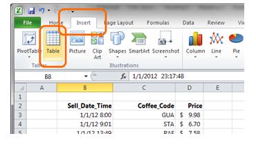
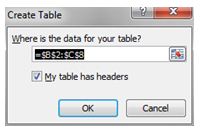
4. Leave the My table has headers checkbox and click Ok
Step 2 – Move the Tables to PowerPivot
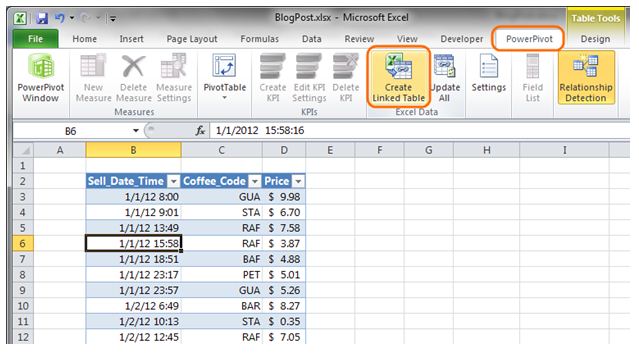
Now we want to move those two tables into PowerPivot where we can link them together. Do the following steps for both tables:
1. Click on any of the cells in one of the tables we just made
2. Click the PowerPivot tab
3. Click the Create Linked Table button
Step 3 – Make the Relationships
Now we want to tell PowerPivot that the Coffee_Code column is related in both our tables. When we crack open the PowerPivot window, we are really looking at the other side of the same coin. I always say that the normal Excel window is one side of the coin, and the PowerPivot window is the other. Both windows are still the same physical file.
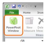
1. Click the PowerPivot Window button
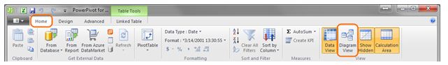
2. Click the Home tab
3. Click the Diagram View button
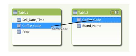
4. Click on and drag one of the Coffee_Codes to the other. Notice how PowerPivot automatically determines the direction of the relationship (very nice for newbies)
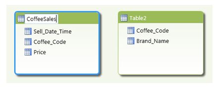
5. Rename Table1 to CoffeeSales and Table2 to CoffeeCodeReference by double clicking the table name
Step 4 – Analyze!
We are now ready to do some analysis on the Excel side of the coin.
1. Click the Excel button to get back to your Excel window

2. At the heart of any good analysis, or chart, is a PivotTable. Click the PowerPivot tab
3. Click the PivotTable button. Note: this is different from the Insert tab’s PivotTable button. By clicking the PivotTable
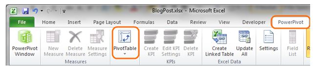
4. Click Ok to create a PivotTable on a new sheet
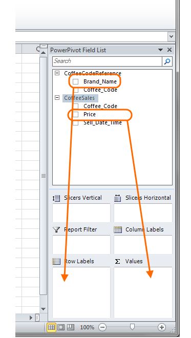
5. Let’s find our sales for each of the brands using the looked up brand names. Drag Brand_Name to the Row Labels section
6. Drag the Price to the Values Section
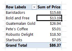
7. Now we have a useful PivotTable that shows the total sales by coffee brand
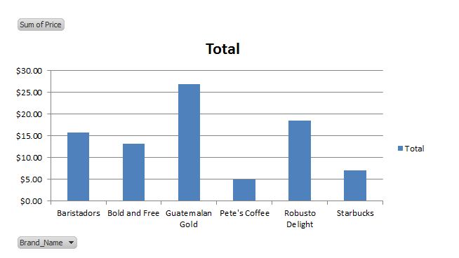
8. Let’s visualize this information by clicking anywhere in the PivotTable.
9. Click the Insert tab
10. Click the Column chart button
Summary
In this post we saw how PowerPivot will smash the need for clunky vlookups. Although we used a small example, PowerPivot is capable of handling millions of rows of data with no problem. The sky is the limit! Actually, your computer’s memory is the limit…